
Lifecycle cost analysis (LCCA) is an economic method that adds up every cost an asset will generate over its service life, discounts those future costs to today’s dollars, and produces a single present-value figure for comparison. The main output is the present-value life-cycle cost, sometimes expressed as net present value (NPV) or equivalent uniform annual cost. You reach for LCCA when you are choosing between mutually exclusive alternatives that trade a lower upfront price against higher long-term spending, or the reverse.
TL;DR:
- Include initial capital, utilities, upkeep, repairs, replacements, and relevant user costs, then subtract residual value; exclude sunk costs and expenses shared by every option.
- Use constant dollar estimates with a real discount rate, or inflated estimates with a nominal rate; mixing them distorts every alternative’s present value.
- Use 30 to 40 years for pavement and 20 to 25 years for buildings and energy equipment, modeling components with shorter lives as replacements.
- Test the discount rate, analysis period, and key cost estimates first; use Monte Carlo analysis when uncertainty is high and alternatives have similar present values.
Table of Contents
- What life-cycle cost analysis covers: cost categories and scope
- Step-by-step LCCA methodology you can implement
- Parameters for present-value analysis: discount rates, inflation, escalation, and analysis period
- Managing uncertainty: sensitivity analysis and probabilistic methods
- Practical applications and worked examples
- GQ-International inputs and project data that speed credible LCCA for PV and energy storage projects
- Integrating LCCA with sustainability and environmental impact assessments
- Best practices for tailoring LCCA to project-specific engineering solutions
- Case studies demonstrating LCCA for photovoltaic mounting systems and guardrails
- Applications of lifecycle cost analysis in transportation safety and renewable energy sectors
- Author perspective: using LCCA responsibly in procurement and project delivery
- How GQ-International supports lifecycle-aware procurement
- FAQ
- Sources
What life-cycle cost analysis covers: cost categories and scope
An LCCA is only as good as the cost categories it captures. Leave out a major cost stream and you bias the comparison toward whichever alternative hides its costs in the category you skipped. The FHWA Life-Cycle Cost Analysis Primer frames this as the core discipline of the method: build a complete, comparable cash flow for each alternative, then let the discounting do the comparison.
For most assets, infrastructure, buildings, and equipment alike, the cost scope includes:
- Initial capital cost: design, procurement, construction, or purchase, including financing costs where relevant.
- Energy and utility costs: electricity, fuel, water, and other recurring consumption costs over the analysis period.
- Operation, maintenance, and repair (OM&R): routine upkeep, inspections, and corrective repairs needed to keep the asset performing.
- Replacement costs: component or system replacements that fall within the analysis period, timed to each item’s expected service life.
- Residual or salvage value: the remaining value of the asset or its components at the end of the analysis period, subtracted from total cost.
For transportation projects, the scope typically widens to include user costs: delay costs from work zones, vehicle operating costs, and in some analyses, crash costs tied to a facility’s safety performance. The FHWA Primer treats these as legitimate agency-plus-user cost components, not an optional add-on, because a cheaper pavement that triggers more frequent lane closures can shift real cost onto the traveling public even when the agency’s own ledger looks favorable.
Two scoping rules keep an LCCA honest. First, exclude sunk costs: money already spent before the decision point does not belong in a forward-looking comparison, no matter how large it was. Second, strip out costs that are identical across every alternative under consideration. If every option requires the same site survey or the same permitting fee, that cost adds nothing to the comparison and only clutters the model. The analysis should isolate differential costs, the ones that actually change depending on which alternative you pick.
Residual value deserves a specific note. An asset rarely reaches zero value the moment the analysis period ends. A pavement overlay might have 10 years of service life left at year 35 of a 35-year analysis; a battery container might retain scrap or secondary-use value. That remaining value gets estimated and subtracted from the discounted cost total, which is one reason two analysts using the same raw cost data can land on noticeably different present-value results if they treat salvage differently.
Step-by-step LCCA methodology you can implement
Running a defensible LCCA is a sequence, not a spreadsheet trick. The procedure below follows the structure the FHWA Primer lays out for transportation projects, generalized so it applies to buildings, equipment, and energy assets as well.
- Define the alternatives and performance requirements. Specify each option in enough technical detail that its service life, maintenance schedule, and capacity are comparable to the others.
- Set the base date and analysis period. The base date anchors your discounting; the analysis period should be long enough to capture at least one major replacement cycle for the shorter-lived alternative.
- Schedule activities and timing. Lay out when construction, maintenance, rehabilitation, and replacement events occur for each alternative across the analysis period.
- Estimate agency costs. Price out initial construction, scheduled maintenance, and replacement events in constant or nominal dollars, consistent with your discounting approach.
- Estimate user costs where relevant. For transportation and other public-facing infrastructure, quantify delay, vehicle operating, and safety-related costs tied to each alternative’s performance and work-zone exposure.
- Assemble the cash flow streams. Place every cost event, agency and user, on a timeline for each alternative so the comparison is complete and chronologically consistent.
- Select a discounting approach and compute present value. Choose a real or nominal discount rate matched to your cost basis, then discount each cash flow to the base date and sum to a present-value life-cycle cost, or convert to equivalent uniform annual cost if that format suits your stakeholders better.
- Analyze results, document assumptions, and present findings. Compare the present-value totals, run sensitivity checks on the assumptions that matter most, and write down every ground rule so a reviewer can reproduce your numbers.
That last step is where many analyses fall short. A result without a documented discount rate, service-life assumption, and cost basis is not reviewable, and an unreviewable LCCA is hard to defend in a procurement dispute or an audit.
Parameters for present-value analysis: discount rates, inflation, escalation, and analysis period
The discount rate and analysis period are the two inputs most likely to flip which alternative wins, so they deserve more scrutiny than any single cost line item.
Real discount rates exclude general inflation and pair with costs expressed in constant dollars; nominal rates include inflation and pair with costs expressed in current, inflated dollars. Mixing the two, a real rate applied to nominal cash flows or vice versa, is one of the most common errors in practice, and it quietly distorts every downstream comparison.
- Match the rate to the cost basis: constant dollars with a real rate, current dollars with a nominal rate, never mixed.
- Pick the analysis period by asset class: pavements commonly run 30 to 40 years, per the FHWA Interim Technical Bulletin, while buildings and major energy equipment often use 20 to 25 years, and shorter-lived components like batteries or inverters get analyzed within that longer envelope through explicit replacement events.
- Use published UPV and UPV factors for energy streams.* The NIST/FEMP annual supplement publishes real and nominal discount rates along with Uniform Present Value (UPV) and modified UPV factors* that convert annual energy costs, adjusted for expected fuel-price escalation, into present-value terms without you having to build an escalation model from scratch.
- Record every ground rule. The discount rate source, analysis period, base date, and price basis all belong in a short assumptions section attached to the results.
Salvage value and remaining service life should be calculated on a consistent basis with the rest of the analysis: if an alternative’s major component has 8 years of useful life left at the end of a 30-year analysis period, prorate its value accordingly rather than assuming either full value or zero.
Managing uncertainty: sensitivity analysis and probabilistic methods
A single-point LCCA result hides how much the answer depends on assumptions you are not fully certain about. Sensitivity analysis and probabilistic simulation expose that hidden fragility before a decision gets locked in.
Sensitivity analysis is the simpler of the two: you vary one input at a time, the discount rate, the analysis period, a maintenance cost estimate, and watch how much the present-value ranking moves. It is fast, requires no special software, and is often enough to show whether a decision is robust or knife-edge.
The FHWA Interim Technical Bulletin recommends probabilistic analysis specifically when input uncertainty is high and the alternatives’ present-value costs are close enough that a single-point comparison could reverse under plausible assumption changes.
- Run sensitivity tests first: they are cheap and quickly flag which assumptions actually matter.
- Escalate to Monte Carlo when alternatives are close: a narrow present-value gap combined with wide input uncertainty is the classic trigger.
- Report percentiles, not just a mean: stakeholders should see the probability that Alternative A beats Alternative B, not only the expected value.
- Flag tail risk explicitly: a low-probability, high-cost outcome (major early failure, steep energy-price escalation) can matter more to a budget holder than the median case.
Pro Tip: Present probabilistic results as a simple chart showing the percentage likelihood that each alternative has the lower life-cycle cost, rather than the raw cost distributions. It reads faster for non-technical decision makers.
Practical applications and worked examples
Cost drivers and realistic analysis periods differ sharply by asset class, which is why a template built for pavement rarely transfers cleanly to a building or an energy project without adjustment.
- Pavement: dominated by initial construction and periodic rehabilitation cost, with user delay cost from work zones often rivaling agency cost on high-traffic corridors.
- Buildings: dominated by energy cost and major system replacement (HVAC, roofing), typically analyzed over 20 to 25 years.
- PV plus battery energy storage (BESS): dominated by inverter and battery replacement timing, since battery chemistry and duty cycle determine when a costly mid-life replacement hits the cash flow.
- Guardrail and safety hardware: dominated by installation cost plus a lower, steadier repair cost tied to crash frequency rather than scheduled maintenance.
A simplified worked example illustrates the mechanics. Say a solar developer is comparing two mounting options for a ground-mount array: Option A costs $100,000 upfront with a 25-year service life and no mid-life replacement; Option B costs $80,000 upfront but requires a $20,000 component replacement in year 15. The lower upfront option remains the better economic choice once the replacement timing and discount rate are both accounted for, though the margin is narrow enough that a sensitivity check on the discount rate and replacement cost would be the sensible next step before committing.
| Asset class | Dominant cost driver | Typical analysis period |
|---|---|---|
| Pavement | Initial construction and rehabilitation | 30–40 years (FHWA) |
| Buildings | Energy use and major system replacement | 20–25 years |
| PV + BESS | Inverter and battery replacement timing | 20–25 years with mid-life replacements |
| Guardrails | Installation and crash-related repair | 20–30 years |
Source project-specific figures, local labor rates, actual energy tariffs, vendor-quoted replacement costs, whenever they are available, and revisit the analysis as those figures firm up rather than treating the first pass as final.
GQ-International inputs and project data that speed credible LCCA for PV and energy storage projects
Populating a PV or BESS life-cycle cost model is often slower than running the model itself, since service-life, replacement-cost, and salvage assumptions all need a credible source. We supply specification-level data across our product lines to help close that gap for analysts working on solar and storage projects.
- Market standing: we have significant market presence in traffic safety products and photovoltaic solutions, with contributions to numerous photovoltaic projects worldwide.
- Mounting system specifications: our GQ-FL series flexible support, GQ-A Series Fixed-Adjustable Mounting System, and GQ-F Series Fixed Mounting System pages list structural and material specifications usable for installation and replacement-cost line items.
- Tracker data: the GQ-T Chaoyang Series Tracker System page details tracking-system specifications relevant to maintenance-interval assumptions.
- Containerized storage inputs: our ODM/OEM Energy Storge Container and Mobile PV-BESS Power Station pages supply specification detail useful for service-life and replacement-timing assumptions in BESS-side LCCA.
These datasheets are a starting point for the engineering review each project still needs before locking in an analysis.
Integrating LCCA with sustainability and environmental impact assessments
Life-cycle cost analysis and life-cycle environmental assessment share a structure, a defined system boundary and a defined time horizon, which makes them natural to run side by side rather than as separate exercises. Pairing them lets a project team see not just which alternative costs less in present-value terms, but whether the lower-cost option also carries a lower embodied-carbon or resource footprint, or whether the two metrics pull in opposite directions.
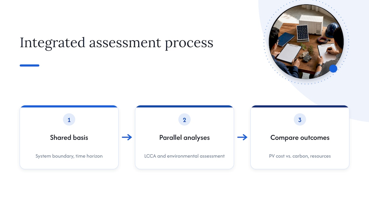
For infrastructure and energy projects, this pairing increasingly shows up in procurement requirements that ask for both an economic and an environmental case. A guardrail system with a longer service life reduces replacement-related material consumption over time, the same factor that lowers its life-cycle cost. A PV mounting structure with lower maintenance needs reduces both site-visit emissions and OM&R spending. When the two assessments are built on the same timeline and the same activity schedule, the environmental data can often reuse the same cost model’s event timing, which saves effort and keeps the two analyses consistent with each other rather than contradicting on when a replacement or major maintenance event actually occurs.
Best practices for tailoring LCCA to project-specific engineering solutions
A generic LCCA template rarely fits a specific project without adjustment, because service lives, maintenance regimes, and failure modes vary by site condition, climate, and load profile. The most useful tailoring starts with matching the cost categories to what the engineering design actually specifies: a coastal installation needs corrosion-related maintenance costs that an inland site does not, and a high-snow-load region needs structural inspection costs that a temperate site can skip.
Tailoring also means adjusting the analysis period and discount rate to match the project’s actual financing and ownership horizon rather than defaulting to a textbook range. A project owner holding an asset for 15 years has a different relevant analysis period than one planning to own it for 40, even if the asset’s physical service life is the same in both cases.
Finally, document every project-specific adjustment alongside the standard ground rules. The FHWA good-practice guidance on LCCA transparency stresses that assumptions, discount rates, and service lives all need to be recorded in a form stakeholders can review, and a tailored analysis has more assumptions to document than a generic one, not fewer.
Case studies demonstrating LCCA for photovoltaic mounting systems and guardrails
Photovoltaic mounting and highway guardrails are two of the clearer illustrations of how LCCA changes a purchasing decision, because both involve a visible upfront price difference against a less visible long-term cost difference. For mounting systems, a lower-cost fixed-tilt structure may look cheaper at installation, while an adjustable or tracking system costs more upfront but can lower the levelized cost of the energy produced over the system’s service life, a tradeoff that only becomes visible once replacement and maintenance costs are discounted alongside the initial price.

For guardrails, the University of California Facilities Manual guidance on life-cycle costing makes the broader point directly: low upfront cost options often carry higher long-term operation, maintenance, and replacement burdens, and a full LCCA is what demonstrates when a higher-quality, higher-cost installation is the economically justified choice rather than the conservative one. A steel guardrail system with better corrosion resistance and a longer service life can carry a higher installation cost than a lighter-gauge alternative, yet show a lower present-value cost once replacement cycles and crash-repair frequency are built into the comparison over a 20 to 30-year analysis period.
Applications of lifecycle cost analysis in transportation safety and renewable energy sectors
In transportation safety, LCCA extends beyond pavement into roadside hardware like guardrails, where the relevant costs include not just installation and periodic replacement but crash-related repair frequency, a cost driver that user-cost-inclusive LCCA, as described in the FHWA Primer, is specifically built to capture. A safety-focused LCCA on a guardrail corridor weighs a higher-strength system’s installation premium against its lower expected repair frequency and longer service interval before replacement.
In renewable energy, LCCA is the standard tool for comparing PV mounting configurations, storage chemistries, and system architectures where the initial capital cost, energy yield, and replacement timing of components like inverters and batteries all move independently of one another. A fixed mounting system and a tracking system can have a similar installed cost per watt while producing different energy yields and different long-term maintenance costs, and only a full life-cycle comparison over the system’s 20 to 25-year horizon separates the better economic choice from the cheaper one.
Author perspective: using LCCA responsibly in procurement and project delivery
LCCA output is a number, not a verdict, and the procurement teams that get the most value from it treat it that way. A present-value figure is only as defensible as the assumptions behind it, which is why documented ground rules and an independent review of the discount rate, analysis period, and service-life estimates matter more than the precision of the final figure itself.
I’d push back on the instinct to treat the lowest-present-value alternative as an automatic winner. Budget constraints, policy requirements, and risk tolerance all belong in the decision alongside the LCCA result, and a probabilistic analysis that shows two alternatives are statistically close should carry more weight than a deterministic one that shows a clear gap built on shaky inputs.
The most useful LCCAs are not one-time exercises. As actual maintenance costs, energy prices, and replacement timing come in, revisiting the model and updating it keeps the analysis honest and gives future procurement decisions a better base to work from.
— Hu
How GQ-International supports lifecycle-aware procurement
Building a life-cycle cost model for a PV, storage, or infrastructure safety project moves faster when the specification and cost inputs come from a single, consistent source rather than being pieced together from scattered vendor sheets. We supply project-ready specification data across mounting, tracking, and containerized storage product lines, letting analysts populate replacement timing and installation cost assumptions without a separate data-collection round for each line item.
- Mounting and tracking specs: our GQ-A Series Fixed-Adjustable Mounting System and GQ-T Chaoyang Series Tracker System pages list the structural detail LCCA models need for installation and maintenance line items.
- Containerized storage specs: our ODM/OEM Energy Storge Container page covers specification inputs relevant to BESS replacement and salvage assumptions.
- Full catalog: browse our complete PV mounting, energy storage, and guardrail product range to match specifications to your project’s analysis period.
If your current model needs project-specific pricing rather than published specifications, request a quote through our OEM and ODM mounting solutions page and we will work from your project’s actual requirements.
For procurement teams also building out construction cost libraries, estimating platforms like ArosBid support the historical unit-price tracking that pairs well with the specification data above when assembling a full LCCA cash flow.
FAQ
How do you calculate lifecycle cost?
You sum the initial cost, energy cost, operation and maintenance cost, and replacement cost, subtract the residual or salvage value, and discount each future cost to the present using a real or nominal discount rate consistent with your cost basis. The result is a single present-value figure you can compare across alternatives, following the structure set out in the FHWA Life-Cycle Cost Analysis Primer.
What are the 5 levels of cost estimation?
Cost estimating frameworks vary by industry and organization, so there is no single universal five-level standard. A common structure moves from a rough order-of-magnitude estimate through conceptual, preliminary, and detailed design-based estimates to a final, bid-ready estimate, with accuracy improving as project definition increases.
What are the four stages of life cycle analysis?
A typical life-cycle analysis moves through defining the alternatives and scope, estimating costs or environmental impacts over the analysis period, discounting or aggregating those values into a comparable total, and analyzing and documenting the results for decision makers. The exact stage names vary by guidance document, but this sequence matches the structure in the FHWA Primer and NIST Handbook 135.
What are the 5 steps of cost-benefit analysis?
A standard cost-benefit analysis defines the alternatives, identifies and quantifies the costs and benefits of each, discounts them to present value, compares the net results, and conducts a sensitivity check before presenting findings. This sequence mirrors the LCCA methodology described above, with the added step of weighing benefits alongside costs rather than comparing costs alone.
Where can I find reliable product specifications for PV mounting LCCA inputs?
Specification pages for mounting and tracking systems, such as our GQ-F Series Fixed Mounting System, list the structural and material detail needed for installation and replacement-cost assumptions. Pairing those specifications with published discount factors from NIST/FEMP gives you both sides of a defensible present-value calculation.
Sources
Credible LCCA work leans on established software and published reference data rather than ad hoc spreadsheets, partly because it is faster and partly because reviewers trust a named methodology.
- Life‑Cycle Cost Analysis Primer (FHWA)
- Life‑Cycle Cost Analysis in Pavement Design (FHWA Interim Technical Bulletin)
- Energy price indices and discount factors (NIST/FEMP supplement)
- NIST Handbook 135 (Life‑Cycle Costing Manual for FEMP)
These references matter beyond convenience: using a named methodology and published discount factors is what lets a procurement reviewer, auditor, or opposing bidder check your numbers against a public standard instead of taking your spreadsheet on faith.